library(tidyverse)
band_members
# A tibble: 3 × 2
name band
<chr> <chr>
1 Mick Stones
2 John Beatles
3 Paul Beatles
band_instruments
# A tibble: 3 × 2
name plays
<chr> <chr>
1 John guitar
2 Paul bass
3 Keith guitar
Joins are powerful functions that allow you to connect two datasets together through matching values. They can be useful with spatial and non-spatial data alike.
Joins rely on “keys” that match records across different datasets. This can be something like a name or ID number.
As a recap of how joins work, we’re going to show a simple example of two different kinds of joins: ‘left’ joins and ‘inner’ joins. For this example, we will be using the band_members
and band_instruments
dataframes, which are simple, 3-row datasets that comes included in the dplyr package.
library(tidyverse)
band_members
# A tibble: 3 × 2
name band
<chr> <chr>
1 Mick Stones
2 John Beatles
3 Paul Beatles
band_instruments
# A tibble: 3 × 2
name plays
<chr> <chr>
1 John guitar
2 Paul bass
3 Keith guitar
As you would expect, the first two arguments in a join function are the two tables you are trying to connect together. The third argument is the “join field”, which is the matching column in both datasets we will use to pair up rows.
A left_join
keeps all of the rows in the first table you specify, appending data from the second table through matching values in the specified “join field”. Let’s see how this kind of join looks with our example data:
<-
band_members_and_instruments left_join(band_members, band_instruments, by = "name")
# When the "join field" column names don't match, you can use:
# by = c("column1" = "column2")
band_members_and_instruments
# A tibble: 3 × 3
name band plays
<chr> <chr> <chr>
1 Mick Stones <NA>
2 John Beatles guitar
3 Paul Beatles bass
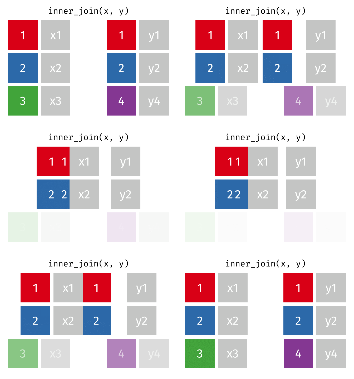
An `inner_join` keeps only the rows that have matching values between both tables in the specified “join field.” Any other rows are discarded. Let’s see how this kind of join looks with our example data:
<-
band_members_with_instruments_only inner_join(band_members, band_instruments, by = "name")
band_members_with_instruments_only
# A tibble: 2 × 3
name band plays
<chr> <chr> <chr>
1 John Beatles guitar
2 Paul Beatles bass
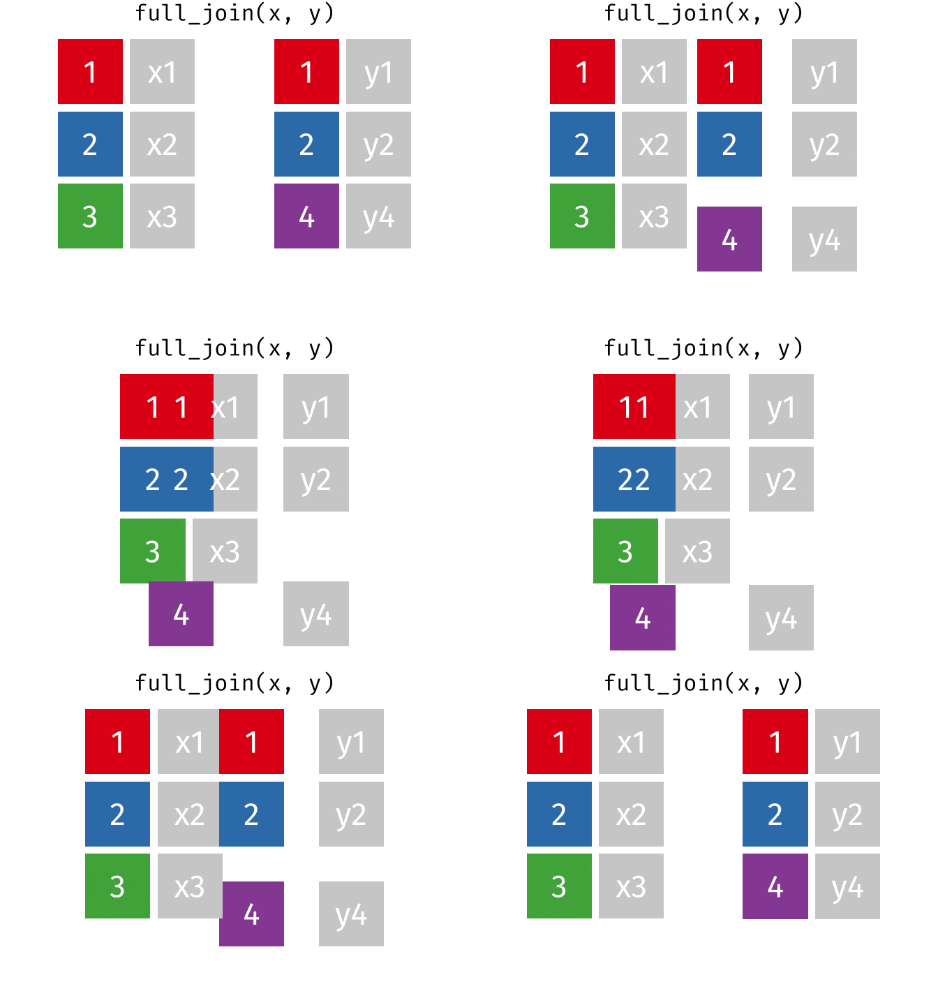
A full_join
keeps all rows from both tables, even if a row from the join field isn’t present in one of them. It shows any missing values as NA.
<-
band_members_with_or_without_instruments full_join(band_members, band_instruments, by = "name")
band_members_with_or_without_instruments
# A tibble: 4 × 3
name band plays
<chr> <chr> <chr>
1 Mick Stones <NA>
2 John Beatles guitar
3 Paul Beatles bass
4 Keith <NA> guitar
Often times, the “join field” in your first table has a different name than that of your second table. For example, you may be trying to join two tables on a common zip code, but the first table calls the column ‘Zip’ and the second table calls it ‘Postal Code’. There’s a special syntax here to make it work:
# Let's change the "name" column to be called "MusicalArtist"
<- band_instruments %>% rename(MusicalArtist = name)
band_instruments_renamed
# In our join function, we need to specify that the "name" column in the first table matches up with the "MusicalArtist" column in the second table. We do that by setting our "by" parameter differently:
<-
band_members_and_instruments_2 inner_join(band_members, band_instruments_renamed,
by = c("name" = "MusicalArtist"))
band_members_and_instruments_2
# A tibble: 2 × 3
name band plays
<chr> <chr> <chr>
1 John Beatles guitar
2 Paul Beatles bass
You can also join across multiple keys (variables), by giving by a list. It will return only rows that match both variables.
Duplicate values in your data can cause problems with joins. For example, what if our `band_instruments` dataset listed “John” twice:
# Let's add a new row to band_instruments… say "John" also plays "flute"
<- band_instruments %>% add_row(name = "John", plays = "flute")
band_instruments_with_dup
# A tibble: 4 × 2
name plays
<chr> <chr>
1 John guitar
2 Paul bass
3 Keith guitar
4 John flute
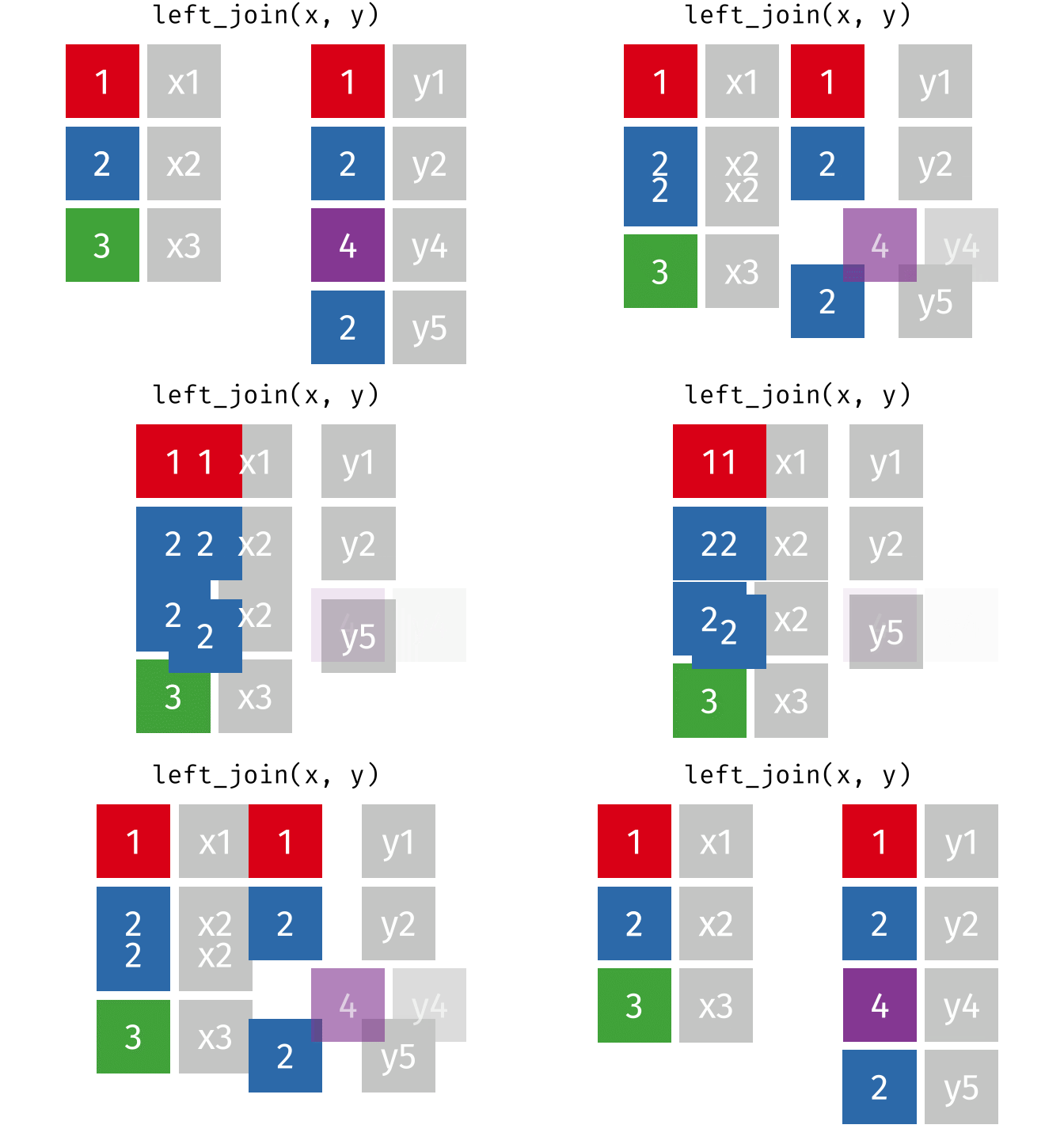
When we try and join our `band_members` table with this new table, we now get 4 rows in the resulting table, even though our first table only had 3 rows… how can that be?
<-
band_members_and_instruments_dup left_join(band_members, band_instruments_with_dup, by = "name")
band_members_and_instruments_dup
# A tibble: 4 × 3
name band plays
<chr> <chr> <chr>
1 Mick Stones <NA>
2 John Beatles guitar
3 John Beatles flute
4 Paul Beatles bass
In R, if there are multiple matches between the two tables, all combinations of the matches are returned. This GIF illustrates visually how this works:
In general, to avoid confusing and unexpected results like this, it’s important to always check for duplicate values in your data, _especially_ in columns that you intend to use as a join field.
Luckily, the `janitor` package has a function for that called `get_dupes`.
library(janitor)# Remember to run `install.packages('janitor')` in your console if you've
%>% get_dupes(name) band_instruments_with_dup
# A tibble: 2 × 3
name dupe_count plays
<chr> <int> <chr>
1 John 2 guitar
2 John 2 flute
Sometimes you may expect duplicate values in a column, and sometimes they may come as a surprise. General Rule: always know what each row represents in your data and what should be unique values.
Sometimes you’ll want to return more rows than you start with, for example if you were matching census divisions to states in order to aggregate the total land area.
#crosswalk between regions and divisions regions_divisions
region division
1 South East South Central
2 West Pacific
3 West Mountain
4 South West South Central
5 Northeast New England
6 South South Atlantic
7 North Central East North Central
8 North Central West North Central
9 Northeast Middle Atlantic
#this doesn't have the region included! oh no! state_area
name division area
1 Alabama East South Central 51609
2 Alaska Pacific 589757
3 Arizona Mountain 113909
4 Arkansas West South Central 53104
5 California Pacific 158693
6 Colorado Mountain 104247
7 Connecticut New England 5009
8 Delaware South Atlantic 2057
9 Florida South Atlantic 58560
10 Georgia South Atlantic 58876
11 Hawaii Pacific 6450
12 Idaho Mountain 83557
13 Illinois East North Central 56400
14 Indiana East North Central 36291
15 Iowa West North Central 56290
16 Kansas West North Central 82264
17 Kentucky East South Central 40395
18 Louisiana West South Central 48523
19 Maine New England 33215
20 Maryland South Atlantic 10577
21 Massachusetts New England 8257
22 Michigan East North Central 58216
23 Minnesota West North Central 84068
24 Mississippi East South Central 47716
25 Missouri West North Central 69686
26 Montana Mountain 147138
27 Nebraska West North Central 77227
28 Nevada Mountain 110540
29 New Hampshire New England 9304
30 New Jersey Middle Atlantic 7836
31 New Mexico Mountain 121666
32 New York Middle Atlantic 49576
33 North Carolina South Atlantic 52586
34 North Dakota West North Central 70665
35 Ohio East North Central 41222
36 Oklahoma West South Central 69919
37 Oregon Pacific 96981
38 Pennsylvania Middle Atlantic 45333
39 Rhode Island New England 1214
40 South Carolina South Atlantic 31055
41 South Dakota West North Central 77047
42 Tennessee East South Central 42244
43 Texas West South Central 267339
44 Utah Mountain 84916
45 Vermont New England 9609
46 Virginia South Atlantic 40815
47 Washington Pacific 68192
48 West Virginia South Atlantic 24181
49 Wisconsin East North Central 56154
50 Wyoming Mountain 97914
<- left_join(regions_divisions, state_area, by = "division")
regions_states
#the join matches state to region and lets us summarize regions_states
region division name area
1 South East South Central Alabama 51609
2 South East South Central Kentucky 40395
3 South East South Central Mississippi 47716
4 South East South Central Tennessee 42244
5 West Pacific Alaska 589757
6 West Pacific California 158693
7 West Pacific Hawaii 6450
8 West Pacific Oregon 96981
9 West Pacific Washington 68192
10 West Mountain Arizona 113909
11 West Mountain Colorado 104247
12 West Mountain Idaho 83557
13 West Mountain Montana 147138
14 West Mountain Nevada 110540
15 West Mountain New Mexico 121666
16 West Mountain Utah 84916
17 West Mountain Wyoming 97914
18 South West South Central Arkansas 53104
19 South West South Central Louisiana 48523
20 South West South Central Oklahoma 69919
21 South West South Central Texas 267339
22 Northeast New England Connecticut 5009
23 Northeast New England Maine 33215
24 Northeast New England Massachusetts 8257
25 Northeast New England New Hampshire 9304
26 Northeast New England Rhode Island 1214
27 Northeast New England Vermont 9609
28 South South Atlantic Delaware 2057
29 South South Atlantic Florida 58560
30 South South Atlantic Georgia 58876
31 South South Atlantic Maryland 10577
32 South South Atlantic North Carolina 52586
33 South South Atlantic South Carolina 31055
34 South South Atlantic Virginia 40815
35 South South Atlantic West Virginia 24181
36 North Central East North Central Illinois 56400
37 North Central East North Central Indiana 36291
38 North Central East North Central Michigan 58216
39 North Central East North Central Ohio 41222
40 North Central East North Central Wisconsin 56154
41 North Central West North Central Iowa 56290
42 North Central West North Central Kansas 82264
43 North Central West North Central Minnesota 84068
44 North Central West North Central Missouri 69686
45 North Central West North Central Nebraska 77227
46 North Central West North Central North Dakota 70665
47 North Central West North Central South Dakota 77047
48 Northeast Middle Atlantic New Jersey 7836
49 Northeast Middle Atlantic New York 49576
50 Northeast Middle Atlantic Pennsylvania 45333
%>%
regions_states group_by(region) %>%
summarize(region_area = sum(area))
# A tibble: 4 × 2
region region_area
<fct> <dbl>
1 Northeast 169353
2 South 899556
3 North Central 765530
4 West 1783960