17. Spatial Features

Author

Patrick Spauster

Video Tutorial

Intro to SF

The Spatial features package allows us to read in spatial data into R and transform it. Let’s get a dataset on [affordable housing production](https://data.cityofnewyork.us/resource/hg8x-zxpr) from the NYC open data portal.

aff_hsg <- read_csv("https://data.cityofnewyork.us/resource/hg8x-zxpr.csv?$limit=10000")

With SF, I can take tabular data and make it into a spatial dataset. In this case I have coordinates that I turn into points us st_as_sf

library(sf)

aff_hsg_sf <- aff_hsg %>% 
  clean_names() %>% 
  filter(!is.na(longitude)) %>%  #remove properties with missing coordinates
  st_as_sf(coords = c("longitude", "latitude"), crs = 2263) #be careful! x = longitude, y = latitude

Plotting SF Objects

Now that this is spatial, I can map it! geom_sf is the ggplot function that maps spatial objects. It works much like any other ggplot.

ggplot()+
  geom_sf(aff_hsg_sf, mapping = aes())

I can use programming for styling, too.

ggplot()+
  geom_sf(aff_hsg_sf,
          mapping = aes(size = all_counted_units,
                        color = all_counted_units),
          alpha = 0.25)

But that doesn’t look very good, let’s add some other layers. I can read in (CDs)[https://data.cityofnewyork.us/resource/5crt-au7u] directly as a shapefile using the geojson version from the Open data portal. This map is a long way from done, but now it has a semblance of a basemap.

cd_sf <- read_sf("https://data.cityofnewyork.us/resource/5crt-au7u.geojson") %>% 
  st_set_crs(st_crs(aff_hsg_sf)) # here I am setting the crs of the new data to the crs of the point data I already have

ggplot()+
  geom_sf(cd_sf,
          mapping = aes())+ #this layer will be on bottom!
  geom_sf(aff_hsg_sf,
          mapping = aes(size = all_counted_units,
                        color = all_counted_units),
          alpha = 0.25) #this layer will be on top!
          #alpha changes the opacity of the dots

I can also summarize data like I would in a tabular dataset

aff_hsg_sum <- aff_hsg %>% 
  group_by(community_board) %>% 
  summarize(total_affordable_units = sum(all_counted_units, na.rm = T))

And then I could create a choropleth with the summarized data, now that I have the nta shapes (just a simple join!)

cd_aff_sum <- cd_sf %>% 
  mutate(community_board = case_when(
    str_sub(boro_cd, 1, 1) == "1" ~ paste0("MN-",str_sub(boro_cd, 2,3)),
    str_sub(boro_cd, 1, 1) == "2" ~ paste0("BX-",str_sub(boro_cd, 2,3)),
    str_sub(boro_cd, 1, 1) == "3" ~ paste0("BK-",str_sub(boro_cd, 2,3)),
    str_sub(boro_cd, 1, 1) == "4" ~ paste0("QN-",str_sub(boro_cd, 2,3)),
    str_sub(boro_cd, 1, 1) == "5" ~ paste0("SI-",str_sub(boro_cd, 2,3)),
  )) %>%  #take the first character of boro_cd, replace it with the boro abbreviation, add the community board number
  left_join(aff_hsg_sum, by = "community_board")

I can map that, now as a choropleth

ggplot()+
  geom_sf(cd_aff_sum,
          mapping = aes(fill = total_affordable_units))

Matching and Crosswalks

I could also match it to other data, and write it out to a shapefile to use in GIS

library(tidycensus)

census_stats <- get_acs(
  geography = "tract",
  variables = c(population = "B01003_001",
                med_income = "B07011_001"),
  year = 2021,
  state = "NY",
  county = c("Bronx", "New York", "Kings", "Queens", "Richmond"),
  output = "wide"
) %>% 
  clean_names()

I need a [crosswalk](https://data.cityofnewyork.us/resource/hm78-6dwm) to go from census tracts to community districts. Open data has one!

cdtas_tracts <- read_csv("https://data.cityofnewyork.us/resource/hm78-6dwm.csv?$limit=10000",
                         col_types = cols(geoid = col_character()))

cdta_stats <- census_stats %>%
  left_join(cdtas_tracts, by = "geoid") %>% 
  group_by(cdtacode, cdtaname) %>% 
  summarize(total_pop = sum(population_e, na.rm = T),
            avg_med_inc = mean(med_income_e, na.rm = T)) %>% 
  mutate()

Now I can join! With everything in the same data frame I can write it out to read into spatial software, or I can visualize it

cd_aff_stats <- cd_aff_sum %>% 
  mutate(cdtacode = str_replace(community_board, "-", "")) %>% 
  left_join(cdta_stats) %>% 
  mutate(aff_units_person = total_affordable_units/total_pop)

st_write(cd_aff_stats,
         "output/cd_aff_hsg.shp",
         append = F)

I can map affordable units per person (normalized!)

ggplot()+
  geom_sf(cd_aff_stats,
          mapping = aes(fill = aff_units_person))

Spatial Operations

What if I wanted to map both both the # of units per cd and the median income?

I can use one of sf’s spatial operators and to take a centroid and map points

points_aff_cd <- cd_aff_stats %>% 
  select(total_affordable_units, cdtacode) %>% 
  st_centroid()

And overlay on a choropleth. You notice that a lot of the buildings are built in low income areas!

ggplot()+
  geom_sf(cd_aff_stats,
          mapping = aes(fill = avg_med_inc))+
  geom_sf(points_aff_cd,
          mapping = aes(size = total_affordable_units),
          color = "pink",
          alpha = 0.5)

I could write out this ggplot to edit in vector graphics

ggsave("output/aff_hsg_inc_nyc.svg")

Spatial Joins

What if I didn’t have a crosswalk and needed to match points to the community district? I can do a spatial join to find what cd all the points fall into.

points_polygons_join <- st_intersection(aff_hsg_sf, cd_sf)

I can then use summarize() to count points in polygons - or do more advanced summaries

points_polygons_join %>% 
  as.data.frame() %>% #summarize works faster without the spatial features attached
  group_by(boro_cd) %>% 
  summarize(points_in_polygon = n(),
            units_per_cd = sum(all_counted_units, na.rm = T))

What if I wanted to find the proportion of affordable housing in the flood zone? I can do this with an intersects and mutate - I don’t even need to join the two datasets!

# floodplain_2020s_100y <- read_sf("https://data.cityofnewyork.us/resource/inra-wqx3.geojson?$limit=10000") %>% 
#   st_make_valid() %>%  #this magic function repairs any invalid geometries
#   st_union() %>% #here I make the entire floodplain into one big shape
#   st_set_crs(st_crs(points_polygons_join)) #and set it to the same crs as my points
# 
# points_polygons_join %>% 
#   mutate(fplain_2020s_100y = lengths(st_intersects(.,floodplain_2020s_100y))) %>%  #st_intersects returns a list of the shapes it intersects with - if its 0 it didn't intersect, if its 1 it did!
#   as.data.frame() %>% 
#   group_by(fplain_2020s_100y) %>% 
#   summarize(count = n(),
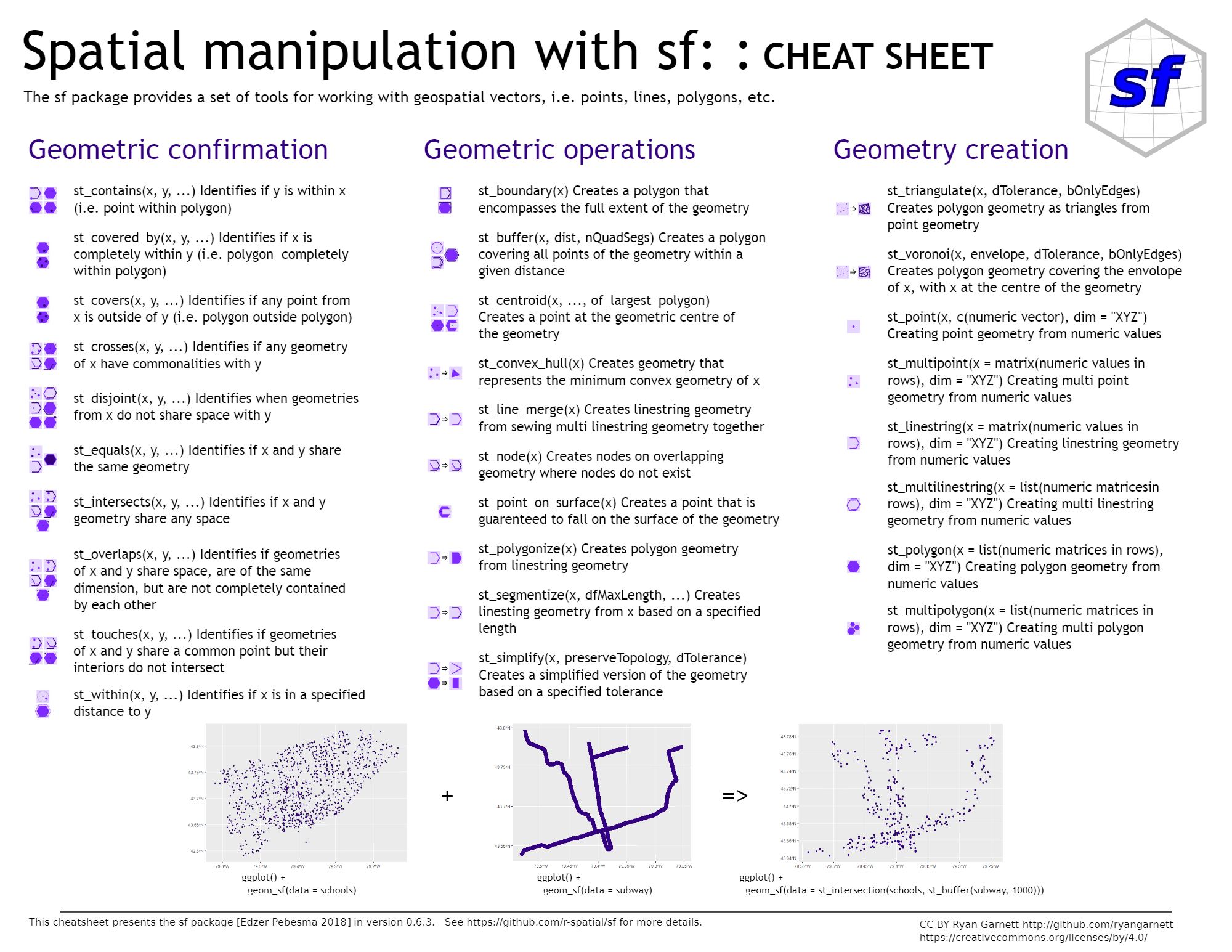
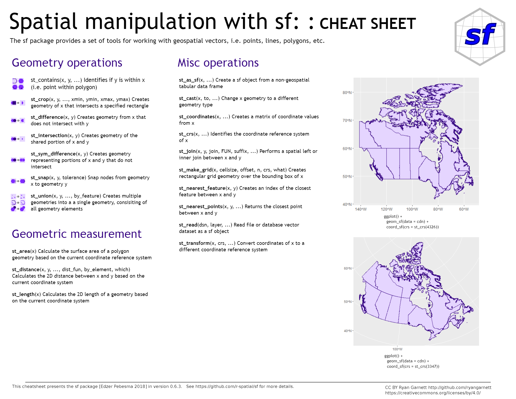
#             units = sum(all_counted_units, na.rm = T))

Cheat Sheet

Many more spatial operations available on the cheat sheets